Long-Term Asset Allocation – The slow return to normal

We expect the economy to ‘normalise’ over the coming years and revert to a situation of under-consumption and under-investment, pushing inflation down to central bank target levels in the US and the UK or lower in Japan and the eurozone. Risk-adjusted returns for a euro-based investor are likely to be modest over the next 10 years.

In a sense, the debate about one of the key drivers of long-term investment returns has not changed over the last several years. Prior to the Covid-19 pandemic, the worry was that major developed market central banks would not be able to reach their inflation targets. The worry is arguably the same today. The key difference, obviously, is that before the pandemic, inflation was below central bank targets, whereas today it is still above target, albeit decreasing.

We believe the US Federal Reserve will be able to return inflation to target despite several new, pro-inflationary factors that have arisen since the pandemic, particularly the acceleration of deglobalisation that began with Donald Trump’s presidency.

As countries and companies strive to produce more goods domestically, or at least closer to home, constrained labour markets are likely to lead to higher prices. Artificial intelligence may help to reduce some of these costs, but the impact will likely not be felt for many years.

A new era of higher inflation and rates  

While we believe inflation will return to target, the new post-pandemic inflationary factors may mean that policy rates will need to be somewhat higher (and economic growth somewhat lower) than they were before. Higher market estimates of the long-run level of the fed funds rate compared to pre-pandemic levels may partly reflect this phenomenon. Whether governments and citizens are happy with the resulting rate of growth and level of unemployment is a separate, political question.

While market expectations of the long-run level of US inflation have certainly risen, they are also in line with central bank targets. Using five-year, five-year USD inflation swaps as a measure of CPI inflation, expectations are 35bp higher on average today than they were before the pandemic (see Exhibit 1).

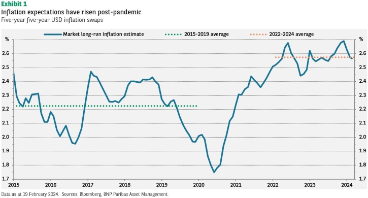
This increase, though, actually aligns with Personal Consumption Expenditure (PCE) inflation stabilising around the Fed’s 2% target. PCE inflation typically runs about 40bp lower than CPI inflation, hence the 2.2% average estimate shown in the chart for 2015-2019 corresponds to below-target PCE inflation at the time. The higher 2.6% inflation forecast today suggest PCE inflation should reach the Fed’s 2% objective.

American resilience…

Aside from higher inflation expectations, there is also the question of potentially higher US GDP growth. The fact that the US economy expanded by 2.5% in 2023 – with the growth rate in the second half of the year sharply higher than in the first half – after an increase in the fed funds rate of 525bp, is astonishing.

The consensus view at the beginning of 2023 for a recession clearly did not sufficiently account for the impact of the USD 1.9 trillion American Rescue Plan and the subsequent Inflation Reduction Act legislation. The higher US growth rate, however, is likely just a temporary boost from fiscal stimulus rather than a permanent change in the long-run potential of US economy. The stimulus was largely financed by an increase in debt (the US has been running a usually large peacetime budget deficit). The resulting higher interest rates will eventually offset the impact of the stimulus.

And Chinese limpness

The other key surprise of 2023 was the disappointing performance of the Chinese stock market (if not necessarily the economy) once zero-Covid restrictions were finally lifted. The economy did expand by 5.2% in 2023, slightly above the government’s target, but the stock market (as measured by the MSCI China index), declined by 12% in 2023 (local currency terms) and has continued to decline this year.

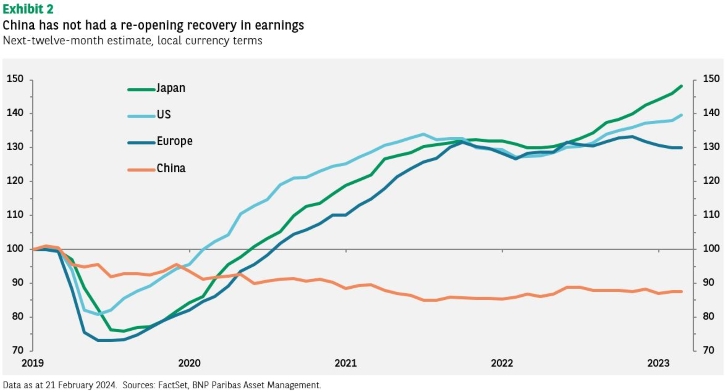
Part of the decline can be explained by a dramatic change in investor sentiment as reflected by a lower price-earnings (P/E) ratio. The forward P/E ratio averaged 12x earnings in the years prior to the pandemic, whereas it has now fallen to below 9x. But an arguably more important factor has been disappointing earnings growth. The expectation was that Chinese companies would see a sizeable increase in earnings with the reopening of the economy, as had been the case in the US and Europe. The hope was that perhaps the increase would be even greater given how much longer and deeper the economy had been locked down.

What perhaps went unappreciated was the damage the lockdowns did to the economy exactly because of their depth and duration, in contrast to relatively brief lockdowns elsewhere. Another factor was the lack of fiscal support provided to households (as opposed to businesses), which meant that savings where either depleted or that households were unwilling to spend then simply because they did not feel they could count on the government for support.

As a result, EPS estimates for the MSCI China index are still 13% below the level prior to the pandemic, when other key markets are at least 30% higher (see Exhibit 2). Profits admittedly never fell as much as they did in other countries, but they have remained depressed. Increased government regulations on key sectors, particularly technology, added further pressure to profit. Until analysts anticipate an increase in profitability, it is difficult to foresee a sustained recovery in Chinese equities.

A decade of modest returns

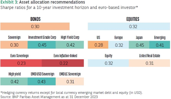
Our expectations for risk-adjusted returns for a euro-based investor over the next 10 years are modest. Few of the assets shown in Exhibit3 have a Sharpe ratio greater than 0.4. 

• Core assets – we are more positive on credit than on rates and equity
• Government bonds – we are marginally more positive on nominal bonds than inflation-linked bonds. We are most negative on euro government bonds. Even though we expect yields to trend down over the coming years, we think this will be accompanied by heightened volatility, leading to a lower Sharpe ratio.
• Private assets provide the potential to further diversify the risks in an investment portfolio; they exploit the ‘illiquidity premium’ as they require a long-term commitment of capital. However, one should be cautious about making simple like-for-like comparisons with public markets as private markets have highly specific characteristics. 

In the appendix (Exhibit 22), you will find a table with expected returns and risks across a broad range of assets and different long-term investment horizons.

Under-consumption and under-investment pushing inflation back

For many of our clients, assets and liabilities both play a key role in their strategic asset allocation decisions. Liabilities are client-specific and therefore typically do not resemble the cash flow pattern of any standard bond index. To incorporate these liabilities into an asset allocation requires a view of the entire yield curve so that the present value and sensitivities to interest rates and inflation shocks of any liability pattern can be calculated.

In other words, we must create a ‘customised bond index’ that closely mimics the interest-rate sensitivities of a client’s liabilities and corresponding matching assets. This approach has the additional benefit of being able to deal with a customized bond index of an asset-only client. Focusing on the term-structure of interest rates provides flexibility in terms of customising our expected returns for fixed-income assets.

More flexibility comes at the price of increased complexity, however. To keep complexity to a minimum, we use a parsimonious yield curve model that only needs a limited number of input parameters to generate the yield curve. A key input for this approach is the 10-year yield.

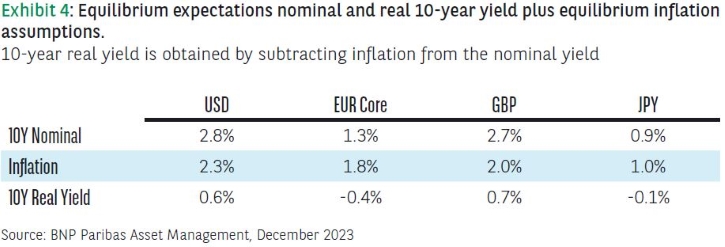
Our base case scenario is that the economic environment will again ‘normalise’ over the coming years, and we will revert back to a situation of under-consumption and under-investment, pushing inflation back to central bank target levels (US and UK) or lower (Japan and eurozone). Demographic headwinds will likely make this an uphill battle for all central banks.

The target 10-year real yield is simply the difference between the 10-year nominal yield and inflation. The lower growth potential in Japan and the eurozone, partly due to ageing populations, in combination with expected under-investment and consumption due to excess savings will likely result, in equilibrium, in small negative real yields for these two regions.

Our framework requires a view on how 10-year nominal and real yields (for inflation-linked bonds) converge from current levels to equilibrium levels. We assume a larger adjustment in the first years (even to the extent of overshooting) after which convergence slows. We then use BNPP AM’s proprietary Monte Carlo (MC) simulation framework to transform the expected convergence path of the (nominal and real) yields into expected return and risk figures.

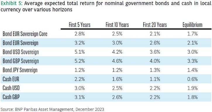
Our base case scenario is that currently tight monetary policy will ease over the coming years, after which yield curves will converge back to lower equilibrium levels. For government bonds and cash this means that for all investment horizons expected returns lie above equilibrium levels. The dislocation for cash is especially high as the current short end of the yield curves lies significantly above the equilibrium rate for all major regions.

Inflation-linked bonds to neutralise inflation risk in part

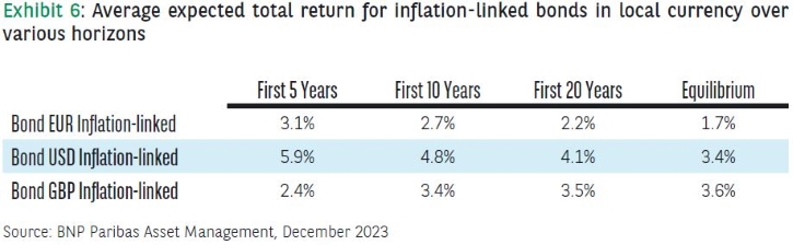
Expected returns of inflation-linked government bonds (in local currency) are detailed in Exhibit 6. Equilibrium returns are slightly higher than nominal bonds for the US and the UK. In the UK, this is mainly caused by the significantly longer maturity of UK inflation-linked bonds.

In the US, inflation-linked bonds are significantly more risky than nominal bonds (consequently pushing up the arithmetic mean in our MC simulation framework used to transform the expected convergence paths of the nominal and real yields into expected return and risk figures).

It is the Sharpe ratio which determines the allocation, and, in equilibrium, it is marginally lower for inflation-linked bonds than for comparable nominal bonds. This is something you would expect as inflation-linked bonds neutralise part of the inflation risk.

For euro and US dollar-denominated bonds, the expected returns for the different investment horizons are higher than the equilibrium returns. This is caused by high current inflation and a real yield curve that is expected to decrease from its current levels, having a positive effect on the price of the current bond portfolio (positive duration effect).

For UK inflation-linked bonds, the opposite holds true – the expected returns for the five to 20-year investment horizon are lower than the equilibrium return. Current inflation is also high in the UK, but this is more than compensated for by a real yield curve that is expected to rise. UK inflation-linked bonds have long maturities (average duration of around 16 years), so a change in real yields has an outsized effect on returns.

Regional preference – UK credit

The modelling approach taken for credit distinguishes between the duration and credit risk components. The return from the duration component simply mirrors the corresponding government bond return. The cash flow pattern of the credit index in combination with the corresponding government bond term-structure is used to calculate the expected return and risk coming from the duration exposure.

Separately, the credit model determines the expected spread return (and risk). Total expected return is simply the sum of the expected return on exposure to duration and credit risk. This is a slight simplification as these components are not exactly linearly separable. However, it typically provides a good approximation and leads to a more intuitive understanding of the build-up of credit returns.

To determine the spread return, current spreads, equilibrium spreads and the probabilities of rating migrations play a key role. For corporate bonds, we believe a focus on default probabilities is too narrow. Especially for investment-grade corporate bonds, a rating downgrade is a bigger risk. Investors often refer to this as the risk of an issuer becoming a ‘fallen angel’. To take this into account, we include Moody’s long-term and forecasted rating migration matrices in our approach.

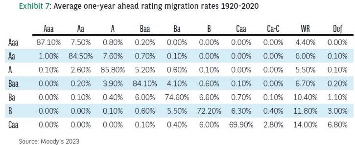
Exhibit 7 shows the average transition matrix for a global corporate bond portfolio from 1920-2022. The rows represent the rating at which a particular corporate issue starts the year; the columns represent the rating at which the issue ends the year. The numbers in the table represent the probability of transitioning from the ‘row-state’ to the ‘column-state’.

For example, the matrix tells us there is a 7.6% probability of any given AAA bond being downgraded to Aa within a year. Consequently, the expected return in any given month on a 10-year AAA bond (for example) is given by combining the yield (or roll-down) effect and the risk of ratings transition or default.

To calculate the yield (or roll-down) effect requires for each region a consideration of the underlying credit curves. For all these credit curves, we construct a current and equilibrium curve in a similar way to the one we constructed for government bonds. The current spread curve moves in future years to the equilibrium curve. As an anchor point of each equilibrium spread curve, we use the median spread for each rating since February 2003. We take the 7-year point as the reference for Investment Grade ratings and the 4-year point for High-Yield ratings.

Exhibit 8 shows the current spread and equilibrium spreads for the target durations. A complicating factor is the rating migration. For example, a AA-rated bond today will not necessarily be a AA-rated bond tomorrow due to default, downgrade or upgrade. Therefore, we use Moody’s current one-year-ahead migration matrix and long-run migration matrix to assess the impact of defaults and rating migrations. In year one, we start with the current one-year-ahead migration matrix and converge in a linear fashion in 10 years to the long-run migration matrix, using from the tenth year onwards the long-run migration matrix.

Exhibits 9 and 10 show the total return in local currency, and the excess return over local cash of credit over various investment horizons for the standard Bloomberg Barclays Aggregate corporate indices.

For all regions, expectations lie above the equilibrium numbers. This is mainly because of higher expectations for the underlying government bonds. The absolute returns for the US and the UK are significantly higher than for their eurozone counterparts. These differences are partly driven by the underlying local cash rates (as can be seen from the numbers in excess over local cash in Exhibit 10).

In excess return (and for hedged return) terms, we have a regional preference for UK credit partly due to higher absolute spread levels for the UK (leading to a larger spread contraction) and higher expectations for the underlying government bonds (over local cash).

EM debt hard currency

As with credit, the expected return for EMD HC consists of a US Treasury or underlying yield and a spread component. Partly due to the limited availability of data, we opt for a more stylised approach than the curve approach used for credit by estimating the historical relationship between the spread over US treasuries for EMD HC. The key explanatory variables are (expected) GDP growth, the average rating for the EMD HC index, and the weighted average US corporate debt spread.

The actual spread and the modelled spread show a closer relationship between 2010 and 2020. We believe the recent history is most representative of the future as emerging markets have become more mature and intertwined with the global economy (this view assumes the impact of the current deglobalisation trend will be limited). The simple spread model, derived from this relationship, allows for the calculation of target spreads conditional on the expected value of the three explanatory variables.

This target spread changes during the first 10 years as the three explanatory variables change. After 10 years, the spread represents the equilibrium spread and does not change further as the explanatory variables are static. The current actual spread typically differs from this target spread.

We assume that this difference between target spread and actual spread disappears in a linear fashion over a 10-year horizon. Combining this target spread and the difference gives the actual (predicted) spread in the next 10 years. This spread is translated into a spread return by simply using the spread duration: i.e.,

Exhibit 11 gives the expected average spread return, US Treasury return and total return at different investment horizons. For the shorter investment horizon, the expected total return for EMD HC lies considerably higher than the equilibrium level: i.e., EMD HC looks ‘undervalued.’ In excess return terms, EMD HC looks overvalued due to spreads being lower than anticipated by our spread model. However, the higher expected returns on US Treasuries more than compensate, leading to higher total return expectations for the shorter investment horizons.

And emerging market local currency debt

The return of EMD Local Currency (LC) can be decomposed into three components: 

• Yield — the income return corresponding to the yield-to-maturity of the index
• Duration — the valuation return corresponding to changes in the yield, and
• Foreign exchange — the return coming from the evolution of EM currencies vs. USD. 

By adding these separate components together, we can closely match the actual total return of the index. This can be seen in Exhibit 13, which shows monthly actual and re-constructed total returns of the JPM GBI EM Global Diversified Composite since 2003.

As can be seen in Exhibit 14, the difference between the yield of EMD LC and the inflation rate of the corresponding EM basket has been relatively stable over the past 20 years, hovering around 2.2%. We assume that, in equilibrium, yields will adhere to this relationship, that is, yield is equal to the average inflation expectation of EM plus a spread.

Starting from the current yield level, the yield converges in 10 years to 6.2% (an equilibrium inflation expectation of 4% plus a 2.2% spread).

Exhibit 15 gives the expected return, at different investment horizons, for the total yield. It also shows average values for different horizons for the duration effect and foreign currencies. The duration effect is calculated using equation (1), while the impact of foreign currency exposure on EMD LC is assessed using Purchasing Power Parity (with adjustment for difference in productivity). In equilibrium, we assume a zero-currency effect.

Equities

To model equity returns we decompose them into the various components — inflation, total yield/income, and real total payout growth — which contribute to the expected return. This approach is often referred to as a total payout model (see Straehl and Ibbotson, 2017, for more details).[1] With the growing importance of buybacks we prefer this approach over the dividend discount model. Additionally, a total payout method has the advantage over an earnings-driven approach in that, unlike earnings, payout is not sensitive to changes in accounting standards.

The total payout model decomposes equilibrium returns into inflation, total yield, and real total payout growth. For inflation, we use the same equilibrium assumption as for fixed income. Consequently, the total payout model for real equity returns becomes the real equilibrium return plus a valuation adjustment:

Real Return = Total Yield + Real Total Payout Growth (adj B.) + Valuation Adjustments (2)

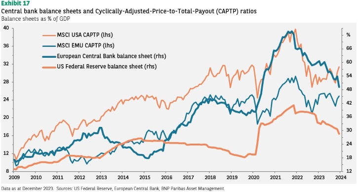
To gauge the valuation component, we look at the variation in the price to total payout (of an index). The starting point is the Cyclically Adjusted Price to Total Payout (CAPTP) ratio, calculated by taking the 10-year median real total payout divided by the current price. The idea is that the current CAPTP will converge to its equilibrium level in 10 years. However, since 2009, we have seen a spectacular increase in the balance sheets of developed economy central banks, which supported an expansion of valuation measures such as the CAPTP.

Exhibit 17 depicts this balance sheet growth versus CAPTP. Regression analyses confirms a relatively significant statistical relationship between central bank balance sheet expansion and CAPTP. These regressions are in-sample, so they do not necessarily confirm the predictive power of balance sheet expansion vis-à-vis equilibrium CAPTP.

With central banks poised to reduce their balance sheets, however, we try to proxy the effect this may have on CAPTP and consequently on the valuation adjustment. We assume current CAPTP will converge to a long-term CAPTP adjusted for each central bank’s balance sheet.

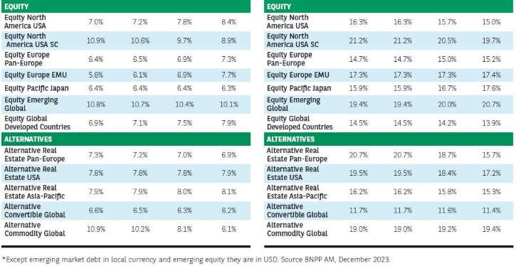
Combining the valuation adjustments with the equilibrium equity expectations over inflation gives real equity return expectations for the first 10 years. Adding the inflation equilibrium assumptions used within the fixed income model gives the total return expectations depicted in Exhibit 16.

For the developed regions, these numbers assume a 30% reduction in central bank balance sheets over the next 10 years, which will depress the valuation component. After last year’s sell-off (partly reversed this year), equities generally still look fairly priced or even cheap. EMU equities are the notable exception.

Real estate

We decompose real estate returns into inflation, income, growth, and valuation components. To proxy the income and growth components, we rely on dividends and earnings. The model for real returns is:

Real Return = Dividend Yield + Real Earnings Growth + Valuation Adjustments (3)

The reason for choosing the dividend model instead of a total payout approach as we do for equities is twofold. Firstly, buybacks are less relevant. A large part of real estate indices consists of real estate investment trusts (REITs), which require payments in dividend for most of their taxable income. Secondly, the data on buybacks is more limited for real estate indices.

Exhibit 18 gives the expected return for real estate over different investment horizons. After the market correction we saw in 2022, real estate looks slightly undervalued.

Diversifying with private assets

Private assets provide the potential to further diversify the risks in an investment portfolio. They exploit the ‘illiquidity premium’ as they require a long-term commitment of capital. Although currently high interest rates have made it slightly more challenging to find good private asset investments, over the long term we believe private assets investing can form a useful addition to a portfolio.

Nonetheless, one must be careful in comparing private and public/liquid assets solely in risk and return terms. For example, a forced sale of a private asset is usually extremely detrimental to performance, meaning there are significant tail risks. Using volatility as the sole measure of risk is therefore not ideal, but to facilitate the comparison with public/liquid assets we use volatility as the reported risk measure, cognisant that this is a simplification.

Exhibits 19 and 20 give the return and risk for a variety of private debt and equity assets. For all private assets there is a difference between committed and actual invested capital. The expected return numbers are for invested capital only. According to Preqin (a private asset index provider) historically around 25% of the capital is not invested. Whether this committed but not invested capital is kept as cash or, say, equity, will have a marked impact on the total expect return.

The risk of private equity is typically not fully reflected in the net asset value (NAV) data. This data is based on a limited number of actual transactions, and hence does not fully reflect the mark-to-market risk.

Capturing the long-term risk of these kinds of investments is critical. Simply looking at the quarterly data, which only contain limited additional information, will likely lead to underestimating this risk. Instead, we try to directly estimate the longer-term risk of these investments.

We explicitly model the risk of a portfolio of buy-and-hold loans with different vintages (i.e., maturing at different dates). The risk measured by volatility is less than that of a bond of similar rating quality but fixed duration: the dominant risk for the latter is rating migration whereas for the former, it is default.

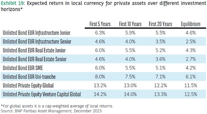
Exhibit 20: Expected risk in local currency for private assets over different investment horizons*

Currency and valuation – To hedge or not?

All risk and return numbers are presented in local terms, avoiding the issue of what an asset’s expected return will be from a particular investor’s currency perspective. As a rule of thumb, we believe an investor should hedge the currency risk of their fixed-income investments as it could otherwise dominate the volatility of their fixed-income exposure.

As a proxy for the hedging cost, we take the difference between US and euro cash returns, resulting in a hedging cost of 0.9%. The expected 4.2% local currency total return for US Treasuries (on a 10-year horizon) becomes a 3.3% euro-hedged return, which is still slightly higher than the 3.0% expected return on euro sovereign government bonds (see Exhibit 5).

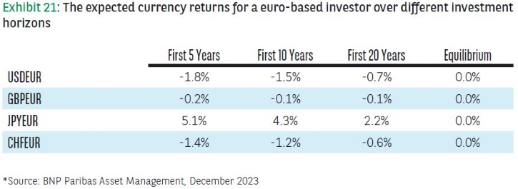
Another factor in determining whether one should hedge foreign currency exposure is the return we can expect on the currency. To address this, we turn to the relative version of the Purchasing Power Parity (PPP) theory of currency determination.

In a world of free trade, the price of identical tradable goods across countries should be normalised by cross-border arbitrage. In other words, nominal exchange rates should move to offset relative changes in price levels. PPP seems to provide a good anchor for foreign exchange forecasts.

The assumption is that if prices in country A rise relative to those in country B, we would expect to see a depreciation of country A’s nominal exchange rate (i.e., a rise in the number of units of currency A necessary to buy one unit of currency B). A recent ECB study comparing equilibrium exchange rate models confirms that in terms of predictability, PPP outperforms two other fair value models.[2]

Exhibit 21 gives the expected currency return from a euro investor’s point of view. In terms of relative purchasing power parity, the US dollar (USD) and Swiss France (CHF) are overvalued versus the euro while the Japanese yen (JPY) is undervalued. Taking into account valuation, hedging cost, but also the extent to which hedging can reduce portfolio risk, we would at the moment typically advise investors to hedge the currency exposure of CHF and USD.

Our approach

The long-term expected return views can be broken down into equilibrium returns and valuation adjustments. The idea is that financial assets typically go through economic cycles. Equilibrium returns represent the return expectations for financial assets over multiple economic cycles. Economic and financial conditions more specific to the current cycle are captured in the valuation adjustment component.

For five to 10-year investment horizons, the valuations component is quite important, whereas for >20-year investment horizons, return expectations are dominated by the equilibrium return. Explicitly separating out the valuation component has the benefit of transparency as it shows how the valuation assumption contributes to the period return.

We have generated these expected return and risk views to facilitate the asset allocation of our clients. Some of our clients have very long liabilities, e.g., the decommissioning of a nuclear power plant could easily lead to liabilities of 50-plus years, or a pension fund with a large number of young participants could have decades-long liabilities.

Having forecasts of long-term returns and risk facilitates the design of a strategic asset allocation to finance these very long-term liabilities.

[1] Philip U Straehl and Roger G. Ibbotson, “The Long-Run Drivers of Stock Returns: Total Payouts and the Real Economy” Financial Analysts Journal, Third Quarter 2017.  

[2] Ca’ Zorzi, Michele and Cap, Adam and Mijakovic, Andrej and Rubaszek, Michał, The Predictive Power of Equilibrium Exchange Rate Models, January 2020. Available at SSRN: https://ssrn.com/abstract=3516749 

Disclaimer